

Staggered Difference-in-Differences#
This notebook demonstrates the StaggeredDifferenceInDifferences estimator in CausalPy, which handles Staggered Difference-in-Differences settings where different units receive treatment at different times.
The Staggered Adoption Problem#
In many real-world settings, treatment is not applied to all units at the same time. Instead, different cohorts of units adopt treatment at different times. This creates a “staggered adoption” pattern.
Why Standard Two-Way Fixed Effects (TWFE) Can Fail#
The standard TWFE regression with a single treatment indicator:
can produce biased estimates in staggered settings [] because:
Already-treated units serve as implicit controls for later-treated units
The estimate is a weighted average of treatment effects that can include negative weights
Dynamic treatment effects (effects that vary over time since treatment) are not properly accounted for
Note
Notice that \(\tau\) in the TWFE formulation above is a scalar—a single number meant to summarize the treatment effect across all units and time periods. This is a fundamental limitation: it assumes the treatment effect is constant, regardless of when a unit was treated or how long they’ve been treated.
Event-study and modern staggered DiD approaches address this by treating treatment effects as dynamic—allowing \(\tau\) to vary by event-time (time relative to treatment). This captures realistic patterns like effects that build up over time, decay, or differ across treatment cohorts.
The Imputation-Based Solution#
CausalPy’s StaggeredDifferenceInDifferences implements the imputation-based estimator of Borusyak et al. [2024]:
Fit a model on untreated observations only - using pre-treatment periods for eventually-treated units plus all periods for never-treated units
Predict counterfactual outcomes for all observations
Compute treatment effects as the difference between observed and predicted outcomes
Aggregate effects by event-time (time relative to treatment) for an event-study curve
Identifying Assumptions#
This estimator relies on three key assumptions:
Absorbing treatment: once a unit is treated, it stays treated in all subsequent periods.
Parallel trends assumption: absent treatment, treated and control units would have followed parallel outcome trajectories.
No anticipation: units do not change behavior in anticipation of future treatment.
If these assumptions are violated, event-time estimates can be biased and causal interpretation may no longer hold. In CausalPy, non-absorbing treatment is rejected during input validation.
import warnings

import matplotlib.pyplot as plt
import numpy as np
import pandas as pd

import causalpy as cp
from causalpy.data.simulate_data import generate_staggered_did_data

warnings.filterwarnings("ignore", category=FutureWarning)
%load_ext autoreload
%autoreload 2
%config InlineBackend.figure_format = 'retina'
Generate Synthetic Staggered Panel Data#
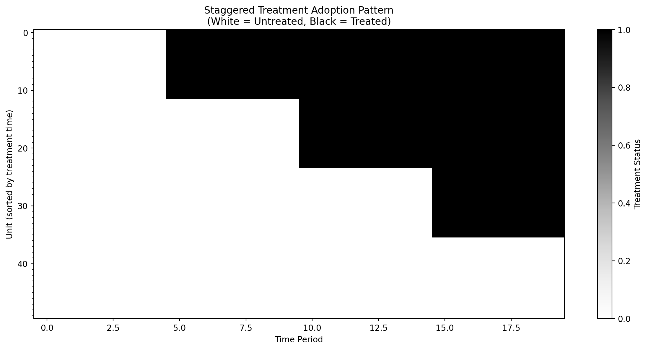
We’ll create synthetic data with:
50 units observed over 20 time periods
3 treatment cohorts adopting at times 5, 10, and 15
Some never-treated units
A known dynamic treatment effect that we can verify
# Define the true treatment effects (dynamic effects that ramp up then stabilize)
# This is used both for data generation and for validating our estimates
TRUE_EFFECTS = {0: 1.0, 1: 1.5, 2: 2.0, 3: 2.5}

# Generate synthetic data with known treatment effects
df = generate_staggered_did_data(
    n_units=50,
    n_time_periods=20,
    treatment_cohorts={5: 12, 10: 12, 15: 12},  # 3 cohorts, 14 never-treated
    treatment_effects=TRUE_EFFECTS,
    unit_fe_scale=2.0,
    time_fe_scale=1.0,
    sigma=0.3,
    seed=42,
)
df.head()
| unit | time | treated | treatment_time | y | y0 | tau | |
|---|---|---|---|---|---|---|---|
| 0 | 0 | 0 | 0 | 15.0 | 0.618468 | 0.898554 | 0.0 |
| 1 | 0 | 1 | 0 | 15.0 | 1.179091 | 1.240722 | 0.0 |
| 2 | 0 | 2 | 0 | 15.0 | -1.132728 | -0.847722 | 0.0 |
| 3 | 0 | 3 | 0 | 15.0 | 0.188053 | 0.289763 | 0.0 |
| 4 | 0 | 4 | 0 | 15.0 | 0.391154 | 0.139062 | 0.0 |
Show code cell source
print(
    f"Panel dimensions: {df['unit'].nunique()} units × {df['time'].nunique()} periods"
)
print(f"Total observations: {len(df)}")
print(f"\nTreatment cohorts:")
print(df.groupby("treatment_time")["unit"].nunique())
Panel dimensions: 50 units × 20 periods
Total observations: 1000

Treatment cohorts:
treatment_time
5.0     12
10.0    12
15.0    12
inf     14
Name: unit, dtype: int64
Visualize the Staggered Treatment Pattern#
Show code cell source
# Create a heatmap of treatment status
fig, ax = plt.subplots(figsize=(12, 6))

# Pivot to get unit x time matrix of treatment status
treatment_matrix = df.pivot(index="unit", columns="time", values="treated")

# Sort by treatment time for better visualization
unit_treatment_times = df.groupby("unit")["treatment_time"].first().sort_values()
treatment_matrix = treatment_matrix.loc[unit_treatment_times.index]

im = ax.imshow(
    treatment_matrix.values,
    aspect="auto",
    cmap="Greys",
    interpolation="nearest",
    vmin=0,
    vmax=1,
)
ax.set_xlabel("Time Period")
ax.set_ylabel("Unit (sorted by treatment time)")
ax.set_title(
    "Staggered Treatment Adoption Pattern\n(White = Untreated, Black = Treated)"
)
from matplotlib.ticker import MultipleLocator

ax.yaxis.set_minor_locator(MultipleLocator(1))
plt.colorbar(im, ax=ax, label="Treatment Status")
plt.tight_layout()
plt.show()
Fit the Staggered DiD Model#
We’ll use a model with unit and time fixed effects, which is the baseline counterfactual model for imputation.
The formula defines a model of untreated potential outcomes. Crucially, this model is fitted only on observations that are not yet treated: pre-treatment periods for units that eventually receive treatment, plus all periods for never-treated units. The fitted model is then used to predict what the treated units would have experienced in the absence of treatment (the counterfactual). Treatment effects are computed as the difference between observed outcomes and these counterfactual predictions.
The formula y ~ 1 + C(unit) + C(time) specifies a two-way fixed effects model, but you’re not limited to this specification. If you have additional covariates that help explain variation in the outcome—such as weather conditions, seasonality indicators, economic indicators, or any other time-varying controls—you can include them in the formula. For example, y ~ 1 + C(unit) + C(time) + temperature + holiday would add temperature and holiday effects to the model. Including relevant covariates can improve the precision of your treatment effect estimates and strengthen the plausibility of the parallel trends assumption.
# Fit the staggered DiD model with PyMC
result = cp.StaggeredDifferenceInDifferences(
    df,
    formula="y ~ 1 + C(unit) + C(time)",
    unit_variable_name="unit",
    time_variable_name="time",
    treated_variable_name="treated",
    treatment_time_variable_name="treatment_time",
    model=cp.pymc_models.LinearRegression(
        sample_kwargs={
            "progressbar": True,
            "random_seed": 42,
        }
    ),
)
Initializing NUTS using jitter+adapt_diag...
Multiprocess sampling (4 chains in 4 jobs)
NUTS: [beta, y_hat_sigma]
Sampling 4 chains for 1_000 tune and 1_000 draw iterations (4_000 + 4_000 draws total) took 2 seconds.
The rhat statistic is larger than 1.01 for some parameters. This indicates problems during sampling. See https://arxiv.org/abs/1903.08008 for details
The effective sample size per chain is smaller than 100 for some parameters. A higher number is needed for reliable rhat and ess computation. See https://arxiv.org/abs/1903.08008 for details
Sampling: [beta, y_hat, y_hat_sigma]
Sampling: [y_hat]
Sampling: [y_hat]
Event-Study Plot#
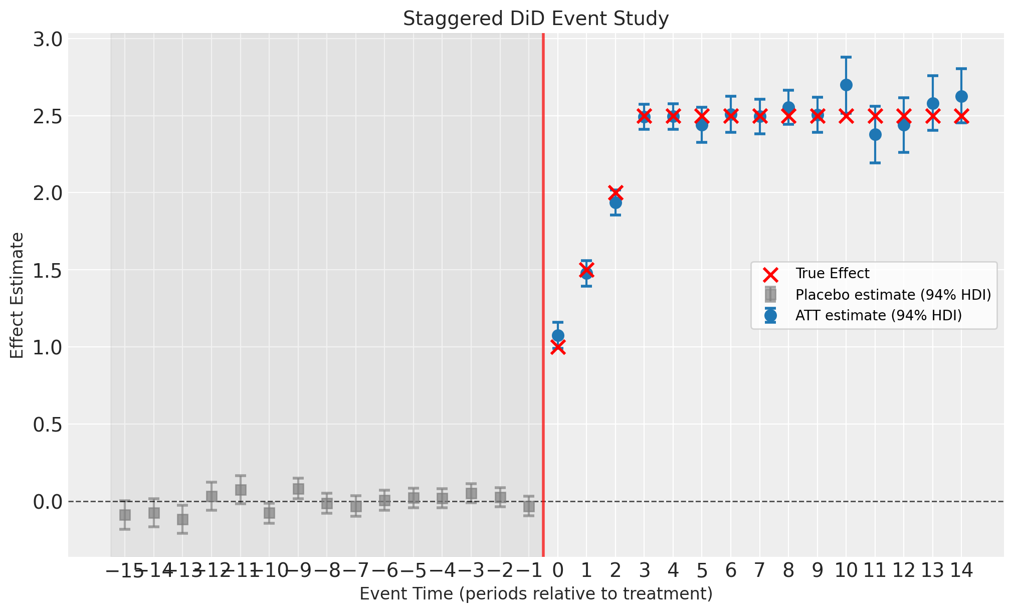
The event-study plot shows estimates at each event-time (time relative to treatment). Key features:
Pre-treatment placebo estimates (event-time < 0, gray squares): These should be close to zero if the parallel trends assumption holds. They are computed as residuals (observed minus predicted) for eventually-treated units before they receive treatment. These are not treatment effects—they are fit diagnostics.
Post-treatment ATT estimates (event-time ≥ 0, blue circles): These are the actual Average Treatment effect on the Treated (ATT) estimates showing the dynamic treatment effect over time since treatment.
Error bars: 94% Highest Density Intervals (HDI) from the Bayesian posterior
Gray shaded region: Pre-treatment period (placebo check zone)
Note
Since we generated synthetic data with known treatment effects, we can overlay the true effects on the plot to validate the estimator’s performance. In real applications, the true effects are unknown.
fig, ax = result.plot()

# Overlay true treatment effects (only possible because we simulated the data)
att_et = result.att_event_time_
post_treatment = att_et[att_et["event_time"] >= 0]
true_vals = [TRUE_EFFECTS.get(e, 2.5) for e in post_treatment["event_time"]]
ax[0].scatter(
    post_treatment["event_time"],
    true_vals,
    color="red",
    marker="x",
    s=100,
    linewidths=2,
    zorder=5,
    label="True Effect",
)
ax[0].legend()

plt.show()
View Summary Statistics#
The n_obs column in the event-time ATT table shows the number of treated unit-time observations contributing to each event-time estimate. This varies across event-times because different cohorts have different lengths of post-treatment history. For example, units treated early in the panel contribute observations at all event-times, while units treated later only contribute to earlier event-times (e.g., event-time 0, 1, 2) before the panel ends.
result.summary(round_to=2)
======================Staggered Difference in Differences=======================
Formula: y ~ 1 + C(unit) + C(time)
Number of units: 50
Number of time periods: 20
Treatment cohorts: [np.float64(5.0), np.float64(10.0), np.float64(15.0)]
Never-treated units: 14

Event-time estimates:
 event_time    type       att  att_lower  att_upper  n_obs
        -15 placebo -0.089727  -0.182651   0.001678     12
        -14 placebo -0.076510  -0.165531   0.015464     12
        -13 placebo -0.117002  -0.208039  -0.026421     12
        -12 placebo  0.030745  -0.059782   0.121330     12
        -11 placebo  0.074539  -0.016959   0.164344     12
        -10 placebo -0.076136  -0.143237  -0.012652     24
         -9 placebo  0.081386   0.014587   0.148938     24
         -8 placebo -0.013679  -0.080336   0.051946     24
         -7 placebo -0.032442  -0.098791   0.033575     24
         -6 placebo  0.004729  -0.060527   0.071197     24
         -5 placebo  0.021254  -0.042810   0.082547     36
         -4 placebo  0.018158  -0.044094   0.081336     36
         -3 placebo  0.051156  -0.011460   0.112558     36
         -2 placebo  0.024409  -0.037726   0.085558     36
         -1 placebo -0.033889  -0.096769   0.030393     36
          0     ATT  1.074842   0.990362   1.159714     36
          1     ATT  1.477406   1.395102   1.559364     36
          2     ATT  1.936514   1.854290   2.016924     36
          3     ATT  2.491325   2.412439   2.572188     36
          4     ATT  2.494277   2.412555   2.577045     36
          5     ATT  2.439444   2.327826   2.554720     24
          6     ATT  2.508034   2.391311   2.625448     24
          7     ATT  2.495111   2.382095   2.607191     24
          8     ATT  2.554547   2.444958   2.666289     24
          9     ATT  2.504438   2.390342   2.620304     24
         10     ATT  2.699058   2.515626   2.879858     12
         11     ATT  2.379267   2.192838   2.562129     12
         12     ATT  2.441211   2.260847   2.617471     12
         13     ATT  2.580254   2.405220   2.759980     12
         14     ATT  2.625220   2.452779   2.803349     12

Model coefficients:
Model coefficients:
    Intercept      0.78, 94% HDI [0.63, 0.95]
    C(unit)[T.1]   -2.6, 94% HDI [-2.9, -2.3]
    C(unit)[T.2]   0.92, 94% HDI [0.62, 1.2]
    C(unit)[T.3]   1.4, 94% HDI [1.2, 1.6]
    C(unit)[T.4]   -4.4, 94% HDI [-4.6, -4.2]
    C(unit)[T.5]   -3.2, 94% HDI [-3.4, -3]
    C(unit)[T.6]   -0.37, 94% HDI [-0.58, -0.18]
    C(unit)[T.7]   -1.1, 94% HDI [-1.3, -0.94]
    C(unit)[T.8]   -0.43, 94% HDI [-0.73, -0.13]
    C(unit)[T.9]   -2.3, 94% HDI [-2.6, -2.1]
    C(unit)[T.10]  1.4, 94% HDI [1.2, 1.5]
    C(unit)[T.11]  1, 94% HDI [0.73, 1.3]
    C(unit)[T.12]  -0.37, 94% HDI [-0.58, -0.18]
    C(unit)[T.13]  1.8, 94% HDI [1.6, 2]
    C(unit)[T.14]  0.34, 94% HDI [0.12, 0.54]
    C(unit)[T.15]  -2.3, 94% HDI [-2.6, -2.1]
    C(unit)[T.16]  0.21, 94% HDI [-0.088, 0.51]
    C(unit)[T.17]  -2.4, 94% HDI [-2.6, -2.2]
    C(unit)[T.18]  1.2, 94% HDI [0.99, 1.5]
    C(unit)[T.19]  -0.7, 94% HDI [-0.89, -0.5]
    C(unit)[T.20]  -0.9, 94% HDI [-1.1, -0.7]
    C(unit)[T.21]  -1.7, 94% HDI [-2, -1.4]
    C(unit)[T.22]  2, 94% HDI [1.8, 2.2]
    C(unit)[T.23]  -0.9, 94% HDI [-1.1, -0.72]
    C(unit)[T.24]  -1.3, 94% HDI [-1.6, -1.1]
    C(unit)[T.25]  -1.3, 94% HDI [-1.6, -0.95]
    C(unit)[T.26]  0.51, 94% HDI [0.27, 0.74]
    C(unit)[T.27]  0.18, 94% HDI [-0.021, 0.37]
    C(unit)[T.28]  0.23, 94% HDI [0.015, 0.43]
    C(unit)[T.29]  0.18, 94% HDI [-0.025, 0.39]
    C(unit)[T.30]  3.7, 94% HDI [3.5, 4]
    C(unit)[T.31]  -1.3, 94% HDI [-1.6, -1.1]
    C(unit)[T.32]  -1.4, 94% HDI [-1.6, -1.2]
    C(unit)[T.33]  -2.1, 94% HDI [-2.3, -1.9]
    C(unit)[T.34]  0.65, 94% HDI [0.35, 0.96]
    C(unit)[T.35]  1.8, 94% HDI [1.5, 2.1]
    C(unit)[T.36]  -0.81, 94% HDI [-1, -0.61]
    C(unit)[T.37]  -2.1, 94% HDI [-2.3, -1.8]
    C(unit)[T.38]  -2.3, 94% HDI [-2.5, -2.1]
    C(unit)[T.39]  0.68, 94% HDI [0.48, 0.87]
    C(unit)[T.40]  0.91, 94% HDI [0.66, 1.1]
    C(unit)[T.41]  0.7, 94% HDI [0.47, 0.93]
    C(unit)[T.42]  -2.1, 94% HDI [-2.3, -1.9]
    C(unit)[T.43]  -0.16, 94% HDI [-0.37, 0.045]
    C(unit)[T.44]  -0.2, 94% HDI [-0.41, 0.0086]
    C(unit)[T.45]  -0.0012, 94% HDI [-0.29, 0.28]
    C(unit)[T.46]  1.1, 94% HDI [0.91, 1.4]
    C(unit)[T.47]  -0.23, 94% HDI [-0.52, 0.066]
    C(unit)[T.48]  0.81, 94% HDI [0.59, 1]
    C(unit)[T.49]  -0.54, 94% HDI [-0.84, -0.25]
    C(time)[T.1]   0.38, 94% HDI [0.26, 0.49]
    C(time)[T.2]   -1.7, 94% HDI [-1.8, -1.6]
    C(time)[T.3]   -0.56, 94% HDI [-0.68, -0.44]
    C(time)[T.4]   -0.77, 94% HDI [-0.89, -0.66]
    C(time)[T.5]   -0.96, 94% HDI [-1.1, -0.84]
    C(time)[T.6]   -0.51, 94% HDI [-0.64, -0.38]
    C(time)[T.7]   1.3, 94% HDI [1.2, 1.4]
    C(time)[T.8]   -1, 94% HDI [-1.1, -0.89]
    C(time)[T.9]   0.72, 94% HDI [0.59, 0.84]
    C(time)[T.10]  -1.9, 94% HDI [-2.1, -1.8]
    C(time)[T.11]  -0.55, 94% HDI [-0.7, -0.42]
    C(time)[T.12]  -0.028, 94% HDI [-0.17, 0.11]
    C(time)[T.13]  0.38, 94% HDI [0.24, 0.53]
    C(time)[T.14]  0.51, 94% HDI [0.37, 0.65]
    C(time)[T.15]  0.45, 94% HDI [0.28, 0.63]
    C(time)[T.16]  -0.61, 94% HDI [-0.79, -0.42]
    C(time)[T.17]  -0.69, 94% HDI [-0.87, -0.5]
    C(time)[T.18]  0.55, 94% HDI [0.37, 0.73]
    C(time)[T.19]  -0.55, 94% HDI [-0.73, -0.37]
    y_hat_sigma    0.31, 94% HDI [0.29, 0.33]
We can get nicely formatted tables from our integration with the maketables package.
from maketables import ETable

ETable(result, coef_fmt="b:.3f")
Effect Summary#
Get a prose summary of the causal effects. The summary includes the average post-treatment effect, and if pre-treatment placebo effects are available, it reports on whether the parallel trends assumption appears to be satisfied:
effect_summary = result.effect_summary()
print(effect_summary.text)
Staggered DiD analysis: The average post-treatment effect across event-times was 2.31 (average 94% HDI [2.19, 2.44]). Pre-treatment placebo check: Average pre-treatment effect was -0.01, consistent with parallel trends assumption. Analysis includes 3 treatment cohort(s).
Pre-Treatment Placebo Check#
The att_event_time_ table includes pre-treatment event times (negative values). These represent the average residuals (observed - predicted) for eventually-treated units before they receive treatment.
Important
Pre-treatment estimates are not ATT (Average Treatment effect on the Treated). They are placebo/fit diagnostics that validate the counterfactual model and parallel trends assumption. If these values are close to zero, it suggests the model fits well and parallel trends is plausible.
# Separate pre- and post-treatment effects
att_et = result.att_event_time_
pre_treatment = att_et[att_et["event_time"] < 0]
post_treatment = att_et[att_et["event_time"] >= 0]

print("Pre-treatment (placebo) effects:")
print(f"  Mean: {pre_treatment['att'].mean():.3f}")
print(f"  Should be close to zero if parallel trends holds")
print()
print("Post-treatment effects:")
print(f"  Mean: {post_treatment['att'].mean():.3f}")
print(f"  True average effect: {np.mean(list(TRUE_EFFECTS.values())):.3f}")
Pre-treatment (placebo) effects:
  Mean: -0.009
  Should be close to zero if parallel trends holds

Post-treatment effects:
  Mean: 2.313
  True average effect: 1.750
Examine the Event-Time ATT Table#
The att_event_time_ attribute provides direct access to the underlying event-time ATT estimates as a pandas DataFrame. This is the same data visualized in the event-study plot, but in tabular form.
When to use this table:
Reporting precise estimates: When you need exact point estimates and credible intervals for a paper or presentation, rather than reading approximate values from a plot.
Custom analysis: When you want to perform additional calculations on the estimates, such as computing cumulative effects, testing specific hypotheses, or comparing effects at particular event-times.
Debugging and validation: When checking that the model is behaving as expected, or comparing estimates across different model specifications.
Exporting results: When you need to save estimates to a file or integrate them into a larger analysis pipeline.
The table includes event_time (periods relative to treatment), type (placebo vs ATT), point estimates (att), credible/confidence intervals, and n_obs (sample size at each event-time).
result.att_event_time_
| event_time | att | att_lower | att_upper | n_obs | |
|---|---|---|---|---|---|
| 0 | -15 | -0.089727 | -0.182651 | 0.001678 | 12 |
| 1 | -14 | -0.076510 | -0.165531 | 0.015464 | 12 |
| 2 | -13 | -0.117002 | -0.208039 | -0.026421 | 12 |
| 3 | -12 | 0.030745 | -0.059782 | 0.121330 | 12 |
| 4 | -11 | 0.074539 | -0.016959 | 0.164344 | 12 |
| 5 | -10 | -0.076136 | -0.143237 | -0.012652 | 24 |
| 6 | -9 | 0.081386 | 0.014587 | 0.148938 | 24 |
| 7 | -8 | -0.013679 | -0.080336 | 0.051946 | 24 |
| 8 | -7 | -0.032442 | -0.098791 | 0.033575 | 24 |
| 9 | -6 | 0.004729 | -0.060527 | 0.071197 | 24 |
| 10 | -5 | 0.021254 | -0.042810 | 0.082547 | 36 |
| 11 | -4 | 0.018158 | -0.044094 | 0.081336 | 36 |
| 12 | -3 | 0.051156 | -0.011460 | 0.112558 | 36 |
| 13 | -2 | 0.024409 | -0.037726 | 0.085558 | 36 |
| 14 | -1 | -0.033889 | -0.096769 | 0.030393 | 36 |
| 15 | 0 | 1.074842 | 0.990362 | 1.159714 | 36 |
| 16 | 1 | 1.477406 | 1.395102 | 1.559364 | 36 |
| 17 | 2 | 1.936514 | 1.854290 | 2.016924 | 36 |
| 18 | 3 | 2.491325 | 2.412439 | 2.572188 | 36 |
| 19 | 4 | 2.494277 | 2.412555 | 2.577045 | 36 |
| 20 | 5 | 2.439444 | 2.327826 | 2.554720 | 24 |
| 21 | 6 | 2.508034 | 2.391311 | 2.625448 | 24 |
| 22 | 7 | 2.495111 | 2.382095 | 2.607191 | 24 |
| 23 | 8 | 2.554547 | 2.444958 | 2.666289 | 24 |
| 24 | 9 | 2.504438 | 2.390342 | 2.620304 | 24 |
| 25 | 10 | 2.699058 | 2.515626 | 2.879858 | 12 |
| 26 | 11 | 2.379267 | 2.192838 | 2.562129 | 12 |
| 27 | 12 | 2.441211 | 2.260847 | 2.617471 | 12 |
| 28 | 13 | 2.580254 | 2.405220 | 2.759980 | 12 |
| 29 | 14 | 2.625220 | 2.452779 | 2.803349 | 12 |
Group-Time ATT Table#
The att_group_time_ attribute provides the most granular level of treatment effect estimates: effects for each combination of treatment cohort (G) and calendar time (t). This is the “building block” data from which event-time effects are aggregated.
Understanding the difference from event-time effects:
Event-time ATT (
att_event_time_): Aggregates effects across cohorts at the same relative time since treatment (e.g., “effect 2 periods after treatment” averages over all cohorts).Group-time ATT (
att_group_time_): Keeps cohort and calendar time separate, showing effects for specific cohort-time pairs (e.g., “effect for cohort treated at t=5, observed at t=7”).
When to use this table:
Cohort heterogeneity analysis: When you suspect treatment effects differ across cohorts (e.g., early adopters vs late adopters respond differently to treatment).
Calendar time effects: When you want to check if treatment effects vary with calendar time, not just time since treatment (e.g., macroeconomic conditions may amplify or dampen effects).
Diagnostics: When event-time effects look suspicious and you want to trace the issue back to specific cohort-time combinations.
Custom aggregation: When you want to compute alternative summary measures (e.g., cohort-specific average effects, or effects weighted by cohort size).
The table includes cohort (treatment time G), time (calendar time t), and treatment effect estimates with uncertainty intervals:
result.att_group_time_.head(20)
| cohort | time | att | att_lower | att_upper | |
|---|---|---|---|---|---|
| 0 | 5.0 | 5 | 1.105831 | 0.981070 | 1.234096 |
| 1 | 5.0 | 6 | 1.313366 | 1.191865 | 1.438411 |
| 2 | 5.0 | 7 | 1.874254 | 1.738034 | 2.002803 |
| 3 | 5.0 | 8 | 2.324531 | 2.195446 | 2.449806 |
| 4 | 5.0 | 9 | 2.495319 | 2.365605 | 2.621871 |
| 5 | 5.0 | 10 | 2.330355 | 2.188604 | 2.468263 |
| 6 | 5.0 | 11 | 2.469498 | 2.326770 | 2.611914 |
| 7 | 5.0 | 12 | 2.452538 | 2.311010 | 2.599357 |
| 8 | 5.0 | 13 | 2.521460 | 2.381104 | 2.661465 |
| 9 | 5.0 | 14 | 2.492747 | 2.348853 | 2.636524 |
| 10 | 5.0 | 15 | 2.699058 | 2.515626 | 2.879858 |
| 11 | 5.0 | 16 | 2.379267 | 2.192838 | 2.562129 |
| 12 | 5.0 | 17 | 2.441211 | 2.260847 | 2.617471 |
| 13 | 5.0 | 18 | 2.580254 | 2.405220 | 2.759980 |
| 14 | 5.0 | 19 | 2.625220 | 2.452779 | 2.803349 |
| 15 | 10.0 | 10 | 0.995009 | 0.864157 | 1.123532 |
| 16 | 10.0 | 11 | 1.493974 | 1.367916 | 1.621203 |
| 17 | 10.0 | 12 | 1.948346 | 1.815420 | 2.081204 |
| 18 | 10.0 | 13 | 2.485107 | 2.350294 | 2.616990 |
| 19 | 10.0 | 14 | 2.378103 | 2.246150 | 2.507052 |
Using scikit-learn Models#
For faster analysis, you can use scikit-learn models instead of PyMC. The error bars represent approximate 95% confidence intervals (±1.96 standard errors).
from sklearn.linear_model import LinearRegression

result_ols = cp.StaggeredDifferenceInDifferences(
    df,
    formula="y ~ 1 + C(unit) + C(time)",
    unit_variable_name="unit",
    time_variable_name="time",
    treated_variable_name="treated",
    treatment_time_variable_name="treatment_time",
    model=LinearRegression(),
)

# Plot the event-study results
fig, ax = result_ols.plot()
plt.show()
The OLS approach produces similar point estimates to the Bayesian model but runs much faster. However, the uncertainty quantification differs: OLS uses asymptotic standard errors while PyMC provides full posterior distributions.
Key Takeaways#
Staggered adoption requires special handling - standard TWFE can produce biased estimates
The imputation approach fits a model on untreated observations and predicts counterfactuals
Event-study curves show dynamic treatment effects and allow for parallel trends checks
Pre-treatment “placebo” estimates (event-time < 0) are not treatment effects—they are fit diagnostics. Values near zero support the parallel trends assumption.
Post-treatment ATT estimates (event-time ≥ 0) are the actual Average Treatment effect on the Treated
CausalPy supports both Bayesian and OLS approaches for flexibility
Sensitivity analysis#
This section walks through pre-treatment placebo diagnostics for staggered DiD using the pipeline API (EstimateEffect → SensitivityAnalysis → GenerateReport). For the shared workflow concepts—Pipeline, pluggable checks, and HTML reports—see Pipeline Workflow.
Pre-treatment placebo check#
The parallel trends assumption is the key identification condition in difference-in-differences: in the absence of treatment, treated and control units would have followed the same trajectory. This assumption cannot be tested directly, but we can probe it by examining pre-treatment event-study estimates — the residuals for eventually-treated units in the periods before they receive treatment [Borusyak et al., 2024].
The PreTreatmentPlaceboCheck formalises this validation. It inspects the pre-treatment event-time ATT estimates already computed by the staggered DiD model and tests whether their mean is close to zero. Since pre-treatment periods should show no treatment effect, systematic deviation from zero suggests a violation of the Parallel trends assumption.
How it works. The check extracts rows with negative event_time from att_event_time_, computes the mean pre-treatment ATT and the maximum absolute pre-treatment ATT, and compares the mean to zero using numpy.isclose with an absolute tolerance proportional to max_abs_pre_att and the threshold argument (default 0.05). The fitted experiment must expose att_event_time_ after EstimateEffect runs.
Walkthrough#
Fit the staggered DiD model (earlier in this notebook or via
EstimateEffectin the pipeline) soatt_event_time_is available.Inspect the event-study plot (above): pre-treatment coefficients should lie near the reference line if parallel trends are plausible.
Run the pipeline cell below with
PreTreatmentPlaceboCheck. EachCheckResultexposestext(human-readable verdict), optionaltable(pre-treatment rows ofatt_event_time_), andmetadata(mean_pre_att,max_abs_pre_att).Open the HTML report (iframe) for a consolidated view next to the main estimates.
Interpreting pass and fail. If the mean pre-treatment ATT is close to zero under the tolerance rule, the check passes, which is consistent with parallel trends in the pre-period. If it fails, treat that as a red flag for misspecification or pre-existing divergence—not as proof that your post-treatment effect estimate is wrong, but as a reason to investigate further. Passing is necessary but not sufficient: it does not guarantee that parallel trends would have held after treatment [].
If this check fails#
A failing PreTreatmentPlaceboCheck means the pre-treatment event-study estimates are not centred on zero, which casts doubt on the parallel trends assumption. Here are concrete steps to diagnose and address the problem:
Inspect the event-study plot for directional pre-trends. Look at the pre-treatment coefficients (gray squares in the plot above). A single noisy estimate far from zero is less concerning than a monotone upward or downward drift across multiple pre-treatment periods. A systematic slope suggests the treated and control groups were already diverging before treatment.
Check whether the pre-treatment window is sparse. If only one or two pre-treatment event-time periods are available, the mean ATT is dominated by sampling noise. In that case, even a “pass” is weak evidence for parallel trends. Consider whether the data can support a longer pre-period or whether additional never-treated units could improve precision.
Revisit the outcome model specification. The imputation estimator’s counterfactual depends on the formula supplied to
StaggeredDifferenceInDifferences. Try adding time-varying covariates (e.g.y ~ 1 + C(unit) + C(time) + covariate) that might absorb differential trends across groups. Also verify that unit and time fixed effects are correctly specified.Compare results under alternative priors with
PriorSensitivity. Re-fit the same staggered specification with tighter or more diffuse priors to check whether the pre-treatment failure is driven by prior-data conflict. If the ATT estimates are robust to reasonable prior variation, the concern is more likely a data/design issue than a modelling artefact.
sensitivity_result = cp.Pipeline(
    data=df,
    steps=[
        cp.EstimateEffect(
            method=cp.StaggeredDifferenceInDifferences,
            formula="y ~ 1 + C(unit) + C(time)",
            unit_variable_name="unit",
            time_variable_name="time",
            treated_variable_name="treated",
            treatment_time_variable_name="treatment_time",
            model=cp.pymc_models.LinearRegression(
                sample_kwargs={"progressbar": True, "random_seed": 42}
            ),
        ),
        cp.SensitivityAnalysis(
            checks=[cp.checks.PreTreatmentPlaceboCheck(threshold=0.05)],
        ),
        cp.GenerateReport(include_plots=True),
    ],
).run()

for cr in sensitivity_result.sensitivity_results:
    print(cr.text)
Initializing NUTS using jitter+adapt_diag...
Multiprocess sampling (4 chains in 4 jobs)
NUTS: [beta, y_hat_sigma]
Sampling 4 chains for 1_000 tune and 1_000 draw iterations (4_000 + 4_000 draws total) took 2 seconds.
The rhat statistic is larger than 1.01 for some parameters. This indicates problems during sampling. See https://arxiv.org/abs/1903.08008 for details
The effective sample size per chain is smaller than 100 for some parameters. A higher number is needed for reliable rhat and ess computation. See https://arxiv.org/abs/1903.08008 for details
Sampling: [beta, y_hat, y_hat_sigma]
Sampling: [y_hat]
Sampling: [y_hat]
Pre-treatment placebo check failed: mean pre-treatment ATT = -0.0089, suggesting possible violation of the parallel trends assumption.
import html as html_module
import warnings

from IPython.display import HTML

with warnings.catch_warnings():
    warnings.filterwarnings(
        "ignore", "Consider using IPython.display.IFrame", UserWarning
    )
    display(
        HTML(
            f'<iframe srcdoc="{html_module.escape(sensitivity_result.report)}" '
            f'width="100%" height="600" style="border:1px solid #ccc;"></iframe>'
        )
    )